この記事では,良く使用される次の5つの窓関数について書く.
- 矩形窓 (Rectangular)
- ハン窓 (Hann)
- ハミング窓 (Hamming)
- ブラックマン窓 (Blackman)
- ブラックマンハリス窓 (Blackman Harris)
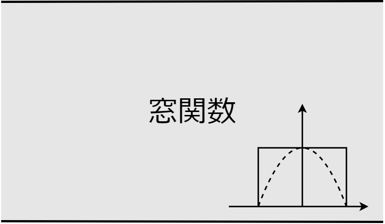
窓関数
窓関数とは,ある区間の信号を取り出すために,もとの信号列からある区間を取り出す際にかけ合わせる関数のこと.
FFT(Fast Fourier Transform)解析をする前には,信号の周期性を確保するためにもとの信号に窓関数をかけてからFFTを行うことが多い.
窓関数 $w$ と信号列 $x$ の積である $wx$ のフーリエ変換結果は,次のように窓関数のフーリエ変換結果$\mathcal{F}(w)$と信号列のフーリエ変換結果$\mathcal{F}(x)$の畳み込みとなる.
$$\mathcal{F}(wx) = \mathcal{F}(w) * \mathcal{F}(x) $$
知りたいのは,$\mathcal{F}(x)$ であるが,数値計算によって得られるのは左辺 $\mathcal{F}(wx)$ のみであるため,$\mathcal{F}(x)$を推定する上で,窓関数 $\mathcal{F}(w)$ の特性は重要になる.
よって,解析する信号の周波数特性を得るためには,解析する信号の特徴に合わせて,窓関数を使い分ける必要がある.
窓関数の種類
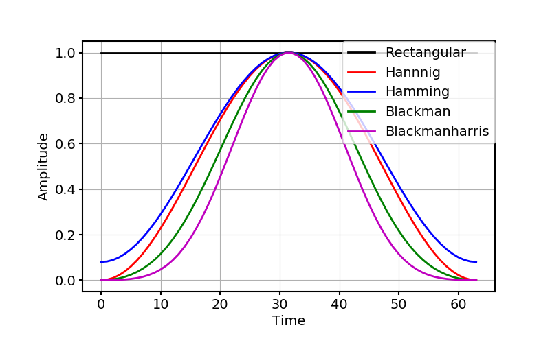
本記事では,次の5つについて扱う.
- 矩形窓 (Rectangular)
- ハン窓 (Hann)
$$w(n) = 0.5 – 0.5 \cos{\left( \frac{2 \pi n}{M} \right)}$$ - ハミング窓 (Hamming)
$$w(n) = 0.54 – 0.46 \cos{\left( \frac{2 \pi n}{M} \right)}$$ - ブラックマン窓 (Blackman)
$$w(n) = 0.42 – 0.5 \cos{\left( \frac{2 \pi n}{M} \right)} + 0.08 \cos{\left( \frac{4 \pi n}{M} \right)}$$ - ブラックマンハリス窓 (Blackman Harris)
$$
\begin{aligned}
w(n) &= 0.42 – 0.48829 \cos{\left( \frac{2 \pi n}{M} \right)} \\
&+ 0.14128 \cos{\left( \frac{4 \pi n}{M} \right)} – 0.01168 \cos{\left( \frac{6 \pi n}{M} \right)}
\end{aligned}
$$
周波数特性
矩形窓,ハン窓,ハミング窓
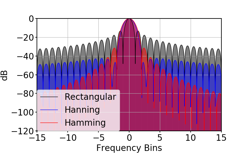
次のグラフは,矩形窓,ハン窓,ハミング窓のFFT結果をプロットしている.
横軸は単位周波数としており,1目盛りがFFTの分解能 $f_{\rm s}/M$ にあたる.
矩形窓は,メインローブが狭いため周波数漏れが少なくなり,周波数分解能が高い.
一方で,サイドローブ成分が高いため,微小な周波数成分の検出には向かない.
ハン窓は,メインローブが広いため,周波数分解能が低いが,サイドローブ成分が低い.
ハミング窓も,同様の特徴があり,メインローブから遠いサイドローブ成分が小さい利点がある.
一方で,メインローブに近いサイドローブ成分が大きい.
ブラックマン窓,ブラックマンハリス窓
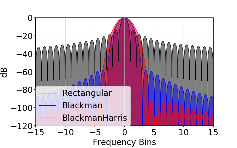
次のグラフは,矩形窓,ブラックマン窓,ブラックマンハリス窓のFFT結果をプロットしている.
ブラックマン窓,ブラックマンハリス窓も同様にメインローブが広く,サイドローブ成分が低い.
まとめ
窓関数の周波数特性について記した.
次の表に,3dB BW(バンド幅)と6dB BW及び,サイドローブの最大値をまとめておく.
メインローブの広さとサイドローブの大きさにはトレードオフの関係があり,目的に応じて窓関数を使い分ける必要がある.
| 窓関数 | 3dB BW (Bins) | 6dB BW (Bins) | Highest SideLobe (dB) |
|---|---|---|---|
| 矩形窓 | 0.89 | 1.21 | -13 |
| ハン窓 | 1.47 | 2.03 | -31 |
| ハミング窓 | 1.32 | 1.84 | -42 |
| ブラックマン窓 | 1.67 | 2.34 | -58 |
| ブラックマンハリス窓 | 1.93 | 2.71 | -90 |
※求め方はスクリプト参照
スクリプト
窓関数のBW(バンド幅)及びサイドローブの最大値の計算スクリプトを書いておく.
import numpy as np
import scipy.signal as signal
import matplotlib.pyplot as plt
from scipy import interpolate

font = {'size' : 20}
plt.rc('font', **font)
plt.rcParams['lines.linewidth']   = 2
plt.rcParams['lines.markersize']  = 10
plt.rcParams['axes.linewidth']    = 1.5
plt.rcParams['xtick.major.width'] = 1.5
plt.rcParams['xtick.minor.width'] = 1
plt.rcParams['ytick.major.width'] = 1.5
plt.rcParams['ytick.minor.width'] = 1

# --------- function ---------- #
def fft(x_ary, fftpt):
    FFT_ary = np.fft.fftshift(np.fft.fft(x_ary, fftpt))
    amp_ary = np.abs(FFT_ary / (len(x_ary)/2))
    FS_ary = amp_ary / np.amax(amp_ary)
    FSdb_ary = 20 * np.log10(FS_ary)
    return FSdb_ary

def getBW(freq_ary, x_ary, mainLobeRange, level):
    logic = np.logical_and(freq_ary >= 0, freq_ary < mainLobeRange)
    index = np.argwhere(logic).T
    interFunc = interpolate.interp1d(x_ary[index].squeeze(),\
                        freq_ary[index].squeeze(), kind='linear')
    return interFunc(level)*2

# --------- param ---------- #
M = 2 ** 6
fftpt = 2 ** 14
plotBottom = -120

label = np.array(['Rectangular', 'Hanning', 'Hamming', 'Blackman', 'BlackmanHarris'])

# --------- main ---------- #
boxcar_ary = signal.boxcar(M)
hann_ary = signal.hann(M)
hamming_ary = signal.hamming(M)
blackman_ary = signal.blackman(M)
blackmanharris_ary = signal.blackmanharris(M)

freqstd_ary =  np.linspace(-M/2, M/2, fftpt)

boxcarSpectrum_ary = fft(boxcar_ary, fftpt)
hannSpectrum_ary = fft(hann_ary, fftpt)
hammingSpectrum_ary = fft(hamming_ary, fftpt)
blackmanSpectrum_ary = fft(blackman_ary, fftpt)
blackmanharrisSpectrum_ary = fft(blackmanharris_ary, fftpt)

## BW
BW3 = np.zeros(5)
BW6 = np.zeros(5)
BW3[0] = getBW(freqstd_ary, boxcarSpectrum_ary, 1, -3)
BW6[0] = getBW(freqstd_ary, boxcarSpectrum_ary, 1, -6)
BW3[1] = getBW(freqstd_ary, hannSpectrum_ary, 2, -3)
BW6[1] = getBW(freqstd_ary, hannSpectrum_ary, 2, -6)
BW3[2] = getBW(freqstd_ary, hammingSpectrum_ary, 2, -3)
BW6[2] = getBW(freqstd_ary, hammingSpectrum_ary, 2, -6)
BW3[3] = getBW(freqstd_ary, blackmanSpectrum_ary, 3, -3)
BW6[3] = getBW(freqstd_ary, blackmanSpectrum_ary, 3, -6)
BW3[4] = getBW(freqstd_ary, blackmanharrisSpectrum_ary, 4, -3)
BW6[4] = getBW(freqstd_ary, blackmanharrisSpectrum_ary, 4, -6)

## sideLobe
sideLobeMax = np.zeros(5)
sideLobeMax[0] = np.amax(boxcarSpectrum_ary[np.argwhere(freqstd_ary > 1)])
sideLobeMax[1] = np.amax(hannSpectrum_ary[np.argwhere(freqstd_ary > 2)])
sideLobeMax[2] = np.amax(hammingSpectrum_ary[np.argwhere(freqstd_ary > 2)])
sideLobeMax[3] = np.amax(blackmanSpectrum_ary[np.argwhere(freqstd_ary > 3)])
sideLobeMax[4] = np.amax(blackmanharrisSpectrum_ary[np.argwhere(freqstd_ary > 4)])

for i in range(len(BW3)):
    print('{} BW -> -3dB:{:.3f}, -6dB:{:.3f} maxSideLobe:{:.3f}\n'\
        .format(label[i],BW3[i], BW6[i], sideLobeMax[i]))


fig, ax = plt.subplots(figsize=(8,5))
fig.subplots_adjust(left=0.15, bottom=0.15)
ax.fill_between(freqstd_ary, plotBottom, boxcarSpectrum_ary, fc='k', alpha=0.5)
ax.fill_between(freqstd_ary, plotBottom, hammingSpectrum_ary, fc='b', alpha=0.5)
ax.fill_between(freqstd_ary, plotBottom, hannSpectrum_ary, fc='r', alpha=0.5)
ax.plot(freqstd_ary, boxcarSpectrum_ary, '-k', label=label[0], lw=1)
ax.plot(freqstd_ary, hammingSpectrum_ary, '-b', label=label[1], lw=1)
ax.plot(freqstd_ary, hannSpectrum_ary, '-r', label=label[2], lw=1)
ax.set_xlim(-15, 15)
ax.set_ylim(plotBottom, 0)
ax.set_xlabel('Frequency Bins')
ax.set_ylabel('dB')
ax.grid()
ax.legend(loc='lower left', borderaxespad=0)
plt.savefig('windowFFT1.png')

fig, ax = plt.subplots(figsize=(8,5))
fig.subplots_adjust(left=0.15, bottom=0.15)
ax.fill_between(freqstd_ary, plotBottom, boxcarSpectrum_ary, fc='k', alpha=0.5)
ax.fill_between(freqstd_ary, plotBottom, blackmanSpectrum_ary, fc='b', alpha=0.5)
ax.fill_between(freqstd_ary, plotBottom, blackmanharrisSpectrum_ary, fc='r', alpha=0.5)
ax.plot(freqstd_ary, boxcarSpectrum_ary, '-k', label=label[0], lw=1)
ax.plot(freqstd_ary, blackmanSpectrum_ary, '-b', label=label[3], lw=1)
ax.plot(freqstd_ary, blackmanharrisSpectrum_ary, '-r', label=label[4], lw=1)
ax.set_xlim(-15, 15)
ax.set_ylim(plotBottom, 0)
ax.set_xlabel('Frequency Bins')
ax.set_ylabel('dB')
ax.grid()
ax.legend(loc='lower left', borderaxespad=0)
plt.savefig('windowFFT2.png')

plt.show()